How to Calculate Break-Even Timelines for Industrial-Scale Mining Operations

Running a mining operation without knowing your break-even point is like driving blindfolded. You might move forward, but you have no idea when you’ll hit profit or crash into losses. Mining engineers and financial analysts face this challenge daily as they evaluate whether a project will generate returns or drain capital for years.

Understanding the Core Components of Mining Break-Even

Break-even analysis answers one critical question: when does your operation stop losing money and start making it?

The calculation seems straightforward. Add up all your costs. Compare them to revenue. Find the intersection point.

Reality is messier.

Mining projects carry unique cost structures that traditional break-even models miss. You’re not selling widgets with predictable margins. You’re extracting minerals from the ground, processing them, and selling commodities whose prices swing 30% in a quarter.

Your cost structure splits into three categories:

Capital expenditures include everything you spend before production starts. Equipment purchases. Infrastructure development. Permitting fees. These costs hit you upfront and don’t repeat annually.

Fixed operating costs continue regardless of production volume. Site maintenance. Security personnel. Administrative overhead. Lease payments. These expenses run even when equipment sits idle.

Variable operating costs scale with production. Energy consumption. Consumables like grinding media. Transportation. Processing chemicals. These costs grow as you mine more ore.

Most analysts make their first mistake here. They lump capital expenditures into annual operating costs, which distorts the timeline. Capital costs should be amortized across the project life, not treated as recurring expenses.

The second mistake involves treating all operating costs as variable. Your electricity bill doesn’t drop to zero when production pauses. Labor contracts don’t vanish during maintenance shutdowns.

Building a Realistic Financial Model

A proper break-even model for industrial mining requires more precision than a basic revenue minus cost equation.

Start with your production schedule. How many tonnes per day? What’s your planned uptime? Most operations assume 90-95% availability, but new facilities often struggle to hit 80% in year one.

Map your ore grade across the mine life. Grade variability changes everything. A 2% copper ore generates different revenue than 1.5% copper, even at identical tonnage.

Calculate recovery rates honestly. Metallurgical testing gives you laboratory results. Actual plant performance typically runs 5-10% lower than lab conditions suggest.

Your revenue calculation needs three inputs:

1. Metal production volume (tonnes of ore × grade × recovery rate)
2. Metal price assumptions (conservative estimates beat optimistic projections)
3. Treatment charges and refining costs (often 10-15% of gross revenue)

Here’s where commodity price volatility enters the picture. Copper prices ranged from $3.50 to $5.00 per pound in 2024. That $1.50 spread represents millions in revenue variation for a 50,000 tonne per year operation.

“The mining projects that survive price crashes are the ones that modeled break-even using bottom-quartile pricing. If you can’t make money at the 25th percentile historical price, you don’t have a viable project.” – Senior mining financial analyst

Calculating Your True Break-Even Timeline

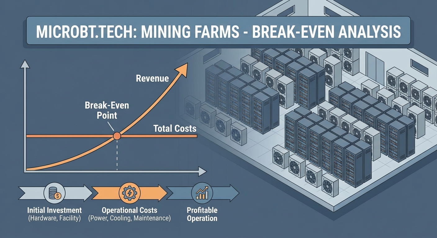
The actual calculation requires tracking cumulative cash flow month by month until it crosses zero.

Month 1 starts deep negative. You’ve spent $50 million on equipment and infrastructure before producing a single tonne of ore. Your cumulative cash flow sits at negative $50 million.

Month 12 shows production ramping up. You’re producing 60% of nameplate capacity. Revenue starts flowing in, but you’re still burning through working capital. Cumulative cash flow might be negative $45 million if you’ve generated $5 million in positive operating cash flow.

Month 24 brings full production. You’re running at 95% capacity. Monthly operating cash flow hits $3 million. Your cumulative position improves to negative $30 million.

Month 36 marks the break-even point. Cumulative cash flow crosses zero. Every dollar after this point represents profit.

This timeline assumes stable prices and smooth operations. Reality introduces complications.

Common Calculation Mistakes That Destroy Accuracy

Even experienced analysts fall into these traps when building break-even models for mining operations.

Mistake	Impact	Correction
Using spot prices for long-term projections	Overestimates revenue by 20-40%	Use 5-year trailing average or futures curve
Ignoring sustaining capital	Understates costs by $2-5M annually	Budget 8-12% of revenue for equipment replacement
Linear production ramp assumptions	Accelerates break-even by 6-12 months	Model S-curve ramp with commissioning delays
Missing working capital requirements	Creates false break-even point	Include inventory, receivables, and payables
Excluding closure costs	Ignores $5-20M future liability	Amortize reclamation across mine life

The working capital mistake deserves special attention. Your operation needs cash on hand to buy consumables, pay workers, and maintain inventory. This capital sits tied up in the business. It doesn’t appear on a simple revenue minus cost calculation, but it delays your actual cash break-even by months.

Sustaining capital represents another hidden cost. That $10 million haul truck doesn’t last forever. Major components need replacement every 5-7 years. Conveyor systems wear out. Processing equipment requires rebuilds. These costs recur throughout mine life.

Sensitivity Analysis for Different Scenarios

No single break-even calculation tells the complete story. You need to model multiple scenarios to understand risk.

Build three core cases:

Base case uses your most likely assumptions. Mid-range metal prices. Planned production rates. Expected operating costs. This scenario shows what happens if everything goes according to plan.

Optimistic case models favorable conditions. Metal prices in the top quartile. Production exceeding nameplate capacity by 5%. Operating costs 10% below budget. This case shows your upside potential.

Conservative case assumes challenges. Bottom quartile pricing. Production at 85% of capacity. Operating costs 15% above budget. This scenario reveals whether the project survives adversity.

The gap between your optimistic and conservative break-even timelines shows your risk exposure. A project that breaks even in month 24 under base assumptions but takes 48 months in the conservative case carries substantial risk.

Price sensitivity matters most. Run the numbers at different metal prices in $0.25 increments. A copper project might break even at month 30 with $4.00 copper but need 50 months at $3.50 copper.

Cost sensitivity comes next. Model what happens if operating costs run 10%, 20%, or 30% above budget. New operations frequently exceed cost estimates during the first year of production.

Production volume sensitivity reveals operational risk. Calculate break-even at 70%, 80%, 90%, and 100% of nameplate capacity. Equipment reliability issues often limit throughput in year one.

The Role of Financing Structure

How you fund the project changes your break-even timeline significantly.

Equity-funded operations have simpler math. You spend the capital. You wait for cumulative cash flow to turn positive. You’re done.

Debt-financed projects add complexity. Interest payments start immediately, even during construction. Principal repayments begin when production starts. Your break-even calculation must include debt service.

A project with $100 million in debt at 8% interest pays $8 million annually just to service the loan. That’s $667,000 per month added to your cost structure before you pay down a dollar of principal.

The debt repayment schedule affects break-even timing. Balloon payments create lumpy cash flows. Amortizing loans spread payments evenly but extend the timeline to positive cash flow.

Some operations use streaming agreements or royalty financing. These structures provide upfront capital in exchange for future production at discounted prices. They reduce initial capital requirements but permanently lower revenue per tonne.

Adjusting for Tax and Depreciation

Tax treatment changes your break-even analysis in ways that surprise many engineers.

Depreciation creates a non-cash expense that reduces taxable income. Your equipment loses value on paper, which lowers your tax bill without affecting cash flow.

A $50 million processing plant depreciated over 10 years generates $5 million in annual depreciation. At a 25% tax rate, that saves $1.25 million in taxes each year.

Loss carryforwards matter for new operations. Your first years run at a loss. Those losses offset future taxable income, reducing your tax burden once the operation turns profitable.

Royalty structures vary by jurisdiction. Some regions charge gross revenue royalties. Others use net profit royalties. The difference affects your break-even calculation by millions.

Gross revenue royalties hit you from day one. A 3% gross royalty on a $100 million annual revenue operation costs $3 million regardless of profitability.

Net profit royalties only apply after you’re profitable. They don’t affect your break-even timeline but reduce returns once you cross that threshold.

Real-World Timeline Expectations

Theory meets reality when you compare calculated break-even timelines against actual mining operations.

Small operations with minimal capital requirements often break even faster. A 500 tonne per day operation processing high-grade ore might reach break-even in 12-18 months if commodity prices cooperate.

Mid-scale operations typically need 24-36 months. These projects carry $50-200 million in capital costs and produce 2,000-5,000 tonnes daily. The larger capital base takes longer to recover.

Large industrial operations frequently require 36-60 months to break even. Projects with $500 million or more in capital costs need years of positive operating cash flow to recover the initial investment.

Underground operations generally take longer than open pit mines. Higher development costs and slower production ramps extend the timeline. An underground copper mine might need 48 months where a comparable open pit operation breaks even in 30 months.

Geographic location influences the timeline through operating costs. Remote sites pay premium wages. Transportation costs eat into margins. Harsh climates increase energy consumption and maintenance expenses.

Commodity type matters. Precious metals operations often break even faster than base metals due to higher margins per tonne. A gold operation might recover capital in 24 months while a zinc operation needs 40 months at similar scale.

Monitoring and Updating Your Analysis

Break-even analysis isn’t a one-time calculation. You need to update it regularly as conditions change.

Track actual performance against your model monthly. Production volumes. Operating costs. Metal prices. Recovery rates. Each variance tells you something about your timeline.

Production below plan extends your break-even date. If you modeled 3,000 tonnes per day but average 2,700, you’re generating 10% less revenue than expected. That pushes break-even out by months.

Operating costs above budget have the same effect. A 15% cost overrun means you need more months of operation to cover the higher expenses.

Metal price changes swing your timeline dramatically. A $0.50 drop in copper prices might extend break-even by 6-12 months for a copper-focused operation.

Update your sensitivity analysis quarterly. Rerun the scenarios with actual performance data. Adjust your assumptions based on what you’ve learned about equipment reliability, ore characteristics, and market conditions.

Some operations discover they’re on track to break even early. Others realize they’re falling behind schedule. Either way, you need accurate information to make decisions about expansion, cost reduction, or financing.

Equipment Selection Impact on Break-Even

The hardware you choose affects both capital costs and operating efficiency, which directly influences your timeline.

Higher efficiency equipment costs more upfront but reduces operating expenses. A premium haul truck might cost 20% more than a basic model but consume 15% less fuel and require less maintenance.

The trade-off calculation depends on your production scale and timeline. For a 10-year mine life, the fuel savings often justify the premium. For a 3-year operation, basic equipment makes more sense.

Processing equipment efficiency matters even more. A mill that achieves 88% recovery versus 85% generates 3% more revenue from the same ore. That difference compounds over years.

Energy efficiency deserves special attention in regions with high power costs. Equipment that reduces energy consumption by 10% might save $2-3 million annually at industrial scale.

Reliability affects break-even through uptime. Equipment that runs 95% of the time versus 85% generates significantly more revenue over a year. The 10% uptime difference translates to 36 additional production days annually.

Maintenance costs vary widely between equipment manufacturers. Some brands require expensive proprietary parts. Others use standard components available locally. The difference shows up in your variable cost structure.

Making Your Numbers Work

Break-even analysis for mining projects requires honest assumptions, detailed modeling, and regular updates. The timeline you calculate guides financing decisions, expansion plans, and risk management strategies.

Start with conservative price assumptions. Model your costs honestly, including sustaining capital and working capital requirements. Build sensitivity scenarios that show what happens when conditions change.

Update your analysis as real performance data replaces assumptions. Track variances monthly and adjust your projections accordingly.

The mining operations that succeed are the ones that know their numbers cold. They understand exactly when they’ll turn profitable and what factors could extend or accelerate that timeline. Your break-even analysis gives you that clarity.